CESM Hierarchical Experiments: From Fully-Coupled Aqua-Planet to Real-world Experiments

I. Ocean Model Modification
II. Coupler Mapping Modification
III. Atmospheric Model Modification
IV. Sea Ice Model Modification
V. Land Model Modification
VI. Appendix

Updated 2020-02-20

The following sketch displays our hierarchical experiments trying to understand the origin of large-scale circulations.

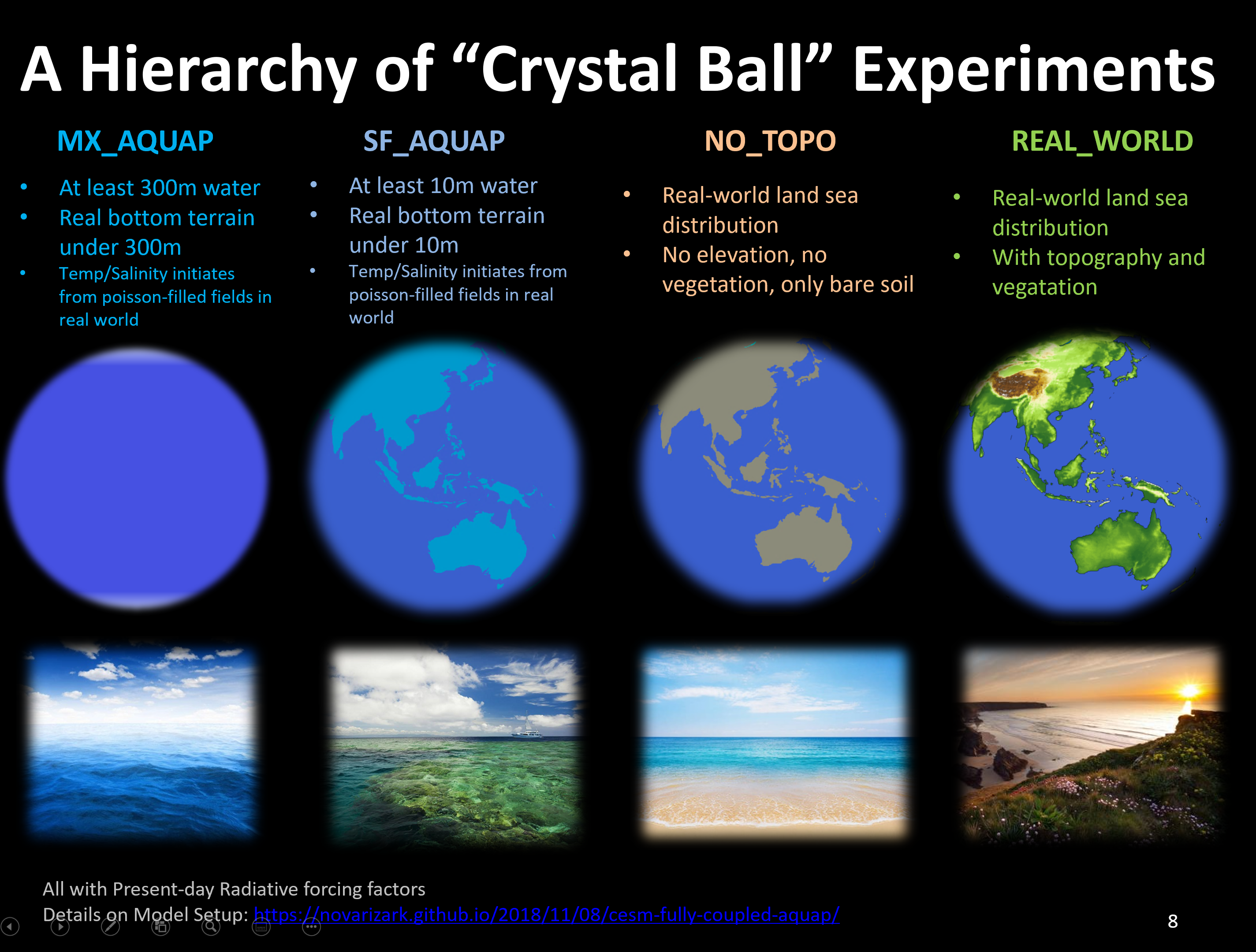
A series of articles archived the procedures to obtain the implementation of the experiments:

Now, finally, we chose the red pill, try to go deep into the model configuration/source, to change the land/sea mask and implement our pure-aqua and surf-aqua experiments.

The implementation of fully coupled aqua-planet experiment is not so straightforward since there is only official support for the prescribed SST aqua-planet. Therefore, as deep-time paleo simulation need to change the land/sea distribution, we seek to use the paleo toolkit to achieve our goal. See reference.

I. Ocean Model Modification

We first begin with the ocean model, POP2. In the guide for deep-time simulation:

The deep time paleo modeler is responsible for creating the binary ocean bottom topography file, the horizontal and vertical ocean grid files, a region mask file, and the ocean initial conditions. In addition, several input template files may need to be changed. For example, if the land/ocean mask is changed, the input template file containing new indices for diagnostic transport calculations will need to be changed. The namelist input file (pop2_in and user_nl_pop2) will need to be changed as well. This section will describe methods that can be used to generate these new files.

Okay, there are four files need to be created.

Binary ocean bottom topography file
Horizontal and vertical ocean grid files
Region mask file
Ocean initial condition

1.1 Binary ocean bottom topography file

In pop2_in, we see the namelist variable define oceanic bottom topography:

topography_file = '/users/yangsong3/CESM/input/ocn/pop/gx1v6/grid/topography_20090204.ieeei4'

This is an IEEE standard 4 byte integer binary file. Since the paleo toolkit for changing the bathymetry is quite complex, we tried to use basic ncl script to change the value.

Results from the file:

(0) min=0   max=60

60 means the deepest ocean bottom lies on the 60th model layer. A list of the ocean depth is attached below:

1: 10m; 2: 20m; 3: 30m; 4: 40m; 5: 50m; 6: 60m; 7: 70m; 8: 80m; 9: 90m; 10: 100m; 11: 110m; 12: 120m; 13: 130m; 14: 140m; 15: 150m; 16: 160m; 17: 170.1968m; 18: 180.7613m; 19: 191.8212m; 20: 203.4993m; 21: 215.9234m; 22: 229.2331m; 23: 243.5845m; 24: 259.1558m; 25: 276.1526m; 26: 294.8147m; 27: 315.4237m; 28: 338.3123m; 29: 363.8747m; 30: 392.5805m; 31: 424.9889m; 32: 461.7666m; 33: 503.7069m; 34: 551.7491m; 35: 606.9967m; 36: 670.7286m; 37: 744.398m; 38: 829.607m; 39: 928.0435m; 40: 1041.368m; 41: 1171.04m; 42: 1318.094m; 43: 1482.901m; 44: 1664.992m; 45: 1863.014m; 46: 2074.874m; 47: 2298.039m; 48: 2529.904m; 49: 2768.098m; 50: 3010.671m; 51: 3256.138m; 52: 3503.449m; 53: 3751.892m; 54: 4001.012m; 55: 4250.525m; 56: 4500.261m; 57: 4750.12m; 58: 5000.047m; 59: 5250.009m; 60: 5499.991m;

Here we set all to Layer 25 49 in PURE_AQUA (2.768km depth), and all land (0) to 1 (10m) in SURF_AQUA model.

However, the NCL had problem when writing the new file (See Appendix01 for details and solution). We change to F90 to realize our goal. For example, below is the code to generate SURF_AQUA bathymetry data:

program change_bathymetry 
    implicit none
    integer, parameter :: fin = 100, fout= 101
    integer, parameter :: nlen = 122880
    integer :: ii
    integer :: status = 0
    integer :: bath(nlen)=0
    character(len=256) :: filename="/users/yangsong3/CESM/input/ocn/pop/gx1v6/grid/topography_20090204.ieeei4"
    character(len=256) :: outname="/users/yangsong3/CESM/input/ocn/pop/gx1v6/grid/topography_surf_aqua_20180607.ieeei4"
    
    open(unit=fin, file=filename, form="unformatted", access="direct", recl=nlen, convert="big_endian")
    read(fin, rec=1) bath 
    close(fin)
    do ii = 1, nlen
        if (bath(ii)<1) then
            bath(ii)=1
        end if
    end do
    open(unit=fout, file=outname, form="unformatted", access="direct", action="write", recl=nlen, convert="big_endian")
    write(fout, rec=1) bath
    close(fout)

end program

Using the above program, we rewrote two files with SURF_AQUA and PURE_AQUA settings.

1.2 Horizontal and vertical ocean grid files

We first check the horizontal grid system.

It can be seen that over the Northern Polar region, the grid system shifts the north pole onto the Greenland Island, and both NH and SH grid poles are located over the landmass.

According to the Paleo FAQ:

The ocean model requires that grid poles be placed over land. Numerically no computation can be done at the convergence point of all longitudes at the grid pole. The ocean model solves this problem by shifting the grid pole away from the geographic pole and placing it over a land mass. (Atmospheric models solve this problem by using numerical filters). Therefore if there is no land at the geographic pole, the numerical pole must be shifted over land elsewhere.

To make it simple, we first tried to maintain the default Greenland replaced grid pole/ SH pole with no land mass. If that does not work, we will try to maintain the Greenland and Antarctica landmass, which will not influence our main results. (The upper test does not work! We have to maintain the polar land inside the ocean grid “black hole”! Otherwise, at the first step of integration, the atmosphere will complain it got a zero longwave radiation (temperature=0K) from the black hole.).

1.3 Region mask file

We check the POP default basin mask file, with the min=-14 and max=11, the masking figure can be found on the NCL popmask page.

And the gx1v6_region_idx is avaliable in the run folder:

IDX	OCEAN NAME
1	‘Southern Ocean ‘
2	‘Pacific Ocean ‘
3	‘Indian Ocean ‘
4	‘Persian Gulf ‘
-5	‘Red Sea ‘
6	‘Atlantic Ocean ‘
7	‘Mediterranean Sea ‘
8	‘Labrador Sea ‘
9	‘GIN Sea ‘
10	‘Arctic Ocean ‘
11	‘Hudson Bay ‘
-12	‘Baltic Sea ‘
-13	‘Black Sea ‘
-14	‘Caspian Sea ‘

Minus-zero Seas are for marginal seas.

We then follow the guide for Deep Time simulation to change the idx:

Deep Time: Since deep time simulations have ocean configurations that differ profoundly from current day, deep time modelers will need to define their own ocean regions. Typically we recommend that they define two simple regions, Northern and Southern Hemisphere.

We change gx1v6_region_idx to:

IDX	OCEAN NAME
1	‘Southern Ocean ‘
2	‘Northern Ocean ‘

region_mask_gx1v6 is modified accordingly.

1.4. Ocean initial condition

The final work is to change the ocean initial condition. For PURE_AQUA and SURF_AQUA, the zonal-mean type should fit well.

ZONAL-MEAN
Initialize with a global, zonally averaged temperature/salinity distribution. POP allows a zonally averaged temperature/salinity file to be used for initialization. This file is binary and the format can be found in the CCSM3/POP source code, subroutine initial.F

Simply change the pop2_in:

init_ts_option = "zonal-mean"

However, it seems that this is a legacy configuration in CCSM3/POP. In POP2, I cannot find the zonal-mean option in the source code, so I conducted a simple test to prove this. Unfortunately, the model does not recognize the settings. Therefore, I have to change the default initial condition to fit the aqua-planet run.

The default initial file for temperature and salinity is ts_PHC2_jan_ic_gx1v6_20090205.ieeer8. Thus, in the SURF_AQUA experiment, we use the poisson grid fill to fill the grid on the ground, and in the PURE_AQUA experiment, we fill all grid with zonal mean and mask out layer deeper than L26.

We should also use the recommended namelist settings for Deep Time Simulations to turn off the processes not so related to the climate physics:

overflows_on = .false.
overflows_interactive = .false.
lhoriz_varying_bckgrnd = .false.
ldiag_velocity = .false.
ltidal_mixing = .false.
bckgrnd_vdc1 = 0.524
bckgrnd_vdc2 = 0.313
sw_absorption_type = 'jerlov'
jerlov_water_type = 3
chl_option = 'file'
chl_filename = 'unknown-chl'
chl_file_fmt = 'bin'

II. Coupler Mapping Modification

All CESM Land/Sea mask info comes from the ocean data. In the paleo resources, we follow the instrudctions to make our mapping and domain data.

Notes:

Scripgrids data available in ${CESM_INPUT}/share/scripgrids/ or download here
Use NCL change gx1v6_090205.nc grid_imask variable

Use following command to generate mapping data:

 ${CESMROOT}/tools/mapping/gen_mapping_files/gen_cesm_maps.sh -fatm /users/yangsong3/CESM/input/share/scripgrids/fv1.9x2.5_090205.nc -natm fv19_25 -focn /users/yangsong3/CESM/input/share/scripgrids/gx1v6_aqua_polar_180614.nc -nocn gx1PT --nogridcheck

Following the instructing in /users/yangsong3/CESM/cesm1_2_2/tools/mapping/gen_domain_files to build gen_domain executable. Note to change the following line in Macro if met MPI/NC variable not found problem:
```
SFC:= mpif90
```

Generate domain files:

./gen_domain -m ../gen_mapping_files/map_gx1PT_TO_fv19_25_aave.180614.nc -o gx1PT -l fv19_25

III. Atmospheric Model Modification

Similar as Coupler generated mapping files, there is a land-sea mask file /users/yangsong3/CESM/input/atm/cam/ocnfrac/domain.camocn.1.9x2.5_gx1v6_090403.nc, using similar technique, change all mask and frac to 1 to present aqua-planet.

IV. Sea Ice Model Modification

Force the model generate sea ice by itself:

Ice initial conditions files are not required for deep time paleoclimate cases. We recommend initializing the ice model with a ‘no ice’ initial state and allowing the model to simulate an ice state. Set ‘no ice’ in the ice model namelist (user_nl_cice).

ice_ic = 'none'

Please see Appendix02 for detailed namelist changes.

V. Land Model Modification

Land model never works in the aqua-planet, so we just use the cpl-generated domain file to drive the model. However, in NO_TOPO series experiments, we reset the surface data to bare ground.

VI. Appendix

6.1 NCL Binary File

We first found that when we use the NCL to write a direct binary file, the file records very large values near the top of the variable type (e.g. 21474836xx for int, and 3e317 for double). Therefore, we tried to use fortran to deal with the problem. Finally, we found this is actually we set the file option as Big_Endian in NCL only for read process. Solution is simple, also set for write process:

setfileoption("bin","WriteByteOrder","BigEndian")

Note to use WriteByteOrder.

6.2 Namelist Changes (SURF_AQUA Final)

env_run.xml

<!--"atm domain file (char) " -->
<entry id="ATM_DOMAIN_FILE"   value="domain.lnd.fv1.9x2.5_gx1v6.aqua.polar.180614.nc"  />
<!--"lnd domain file (char) " -->
<entry id="LND_DOMAIN_FILE"   value="domain.lnd.fv1.9x2.5_gx1v6.aqua.polar.180614.nc"  />
<!--"ice domain file (char) " -->
<entry id="ICE_DOMAIN_FILE"   value="domain.ocn.gx1v6.aqua.polar.180614.nc"  />
<!--"ocn domain file (char) " -->
<entry id="OCN_DOMAIN_FILE"   value="domain.ocn.gx1v6.aqua.polar.180614.nc"  />

<!--"atm2ocn flux mapping file (char) " -->
<entry id="ATM2OCN_FMAPNAME"   value="cpl/gridmaps/fv1.9x2.5/map_fv19_25_TO_gx1v6_aave.aqua.polar.180614.nc"  />
<!--"atm2ocn state mapping file (char) " -->
<entry id="ATM2OCN_SMAPNAME"   value="cpl/gridmaps/fv1.9x2.5/map_fv19_25_TO_gx1v6_blin.aqua.polar.180614.nc"  />
<!--"atm2ocn vector mapping file (char) " -->
<entry id="ATM2OCN_VMAPNAME"   value="cpl/gridmaps/fv1.9x2.5/map_fv19_25_TO_gx1v6_patc.aqua.polar.180614.nc"  />
<!--"ocn2atm flux mapping file (char) " -->
<entry id="OCN2ATM_FMAPNAME"   value="cpl/gridmaps/gx1v6/map_gx1v6_TO_fv19_25_aave.aqua.polar.180614.nc"  />
<!--"ocn2atm state mapping file (char) " -->
<entry id="OCN2ATM_SMAPNAME"   value="cpl/gridmaps/gx1v6/map_gx1v6_TO_fv19_25_aave.aqua.polar.180614.nc"  />

user_nl_pop2

init_ts_file = '/users/yangsong3/CESM/input/ocn/pop/gx1v6/ic/ts_surf_aqua_polar_PHC2_jan_ic_gx1v6_20180613.ieeer8'
region_mask_file = '/users/yangsong3/CESM/input/ocn/pop/gx1v6/grid/region_mask_aqua_polar_20180612.ieeei4'
region_info_file = '/users/yangsong3/CESM/cesm1_2_2/models/ocn/pop2/input_templates/gx1v6_aqua_region_ids'
topography_file = '/users/yangsong3/CESM/input/ocn/pop/gx1v6/grid/topography_surf_aqua_polar_20180607.ieeei4'
n_transport_reg = 1
diag_transp_freq_opt='never'
diag_transport_file='/users/yangsong3/CESM/cesm1_2_2/models/ocn/pop2/input_templates/gx1v6_transport_contents_aqua'

!-- dt_count sets the number of times the ocean is coupled per NCPL_BASE_PERIOD.
dt_count=30

overflows_on = .false.
overflows_interactive = .false.
lhoriz_varying_bckgrnd = .false.
ldiag_velocity = .false.
ltidal_mixing = .false.

!--The new background vertical velocity parameters were determined by Gokhan and Christine to increase Kappa-v in the deeper ocean in absence of tidal mixing. The tidal mixing normally would do this.
bckgrnd_vdc1 = 0.524
bckgrnd_vdc2 = 0.313

sw_absorption_type = 'jerlov'
jerlov_water_type = 3
chl_option = 'file'
chl_filename = 'unknown-chl'
chl_file_fmt = 'bin'

user_nl_atm

bnd_topo       = '/users/yangsong3/CESM/input/atm/cam/topo/USGS-gtopo30_1.9x2.5_pure.nc' 
ncdata='/users/yangsong3/L_Zealot/B/B20f19-surf-aqua/indata/B20f19-topo.cam.i.0010-01-01-00000.nc'
!dtime=900

user_nl_clm

finidat = '/users/yangsong3/L_Zealot/B/B20f19-surf-aqua/indata/B20f19-surf-aqua.clm2.r.0001-01-06-00000.nc' 
fsurdat = '/users/yangsong3/CESM/input/lnd/clm2/surfdata/surfdata_1.9x2.5_bare_ground_simyr2000_c091005.nc'
urban_hac='OFF'

user_nl_cice

kmt_file = '/users/yangsong3/CESM/input/ocn/pop/gx1v6/grid/topography_surf_aqua_polar_20180607.ieeei4'
ice_ic = 'none'
xndt_dyn = 2

user_nl_rtm

finidat_rtm=''

6.3 Error Log

6.3.1 Polar Land

POP aborting… (init_moc_ts_transport_arrays) no transport regions have been detected – che ck namelist transports_nml

It seems the ocean transport diag met some problems.

The transport_contents input_template is used for diagnostic purposes only. In this file, the modeler can specify ocean locations (straits for example) for ocean transport computations that will be output in the ocean log files.

I first tried to create my own transport_contents file, and we met end-of-file read crashes. It is clear that the number of diag locations is hard-coded in the model source code. So I then tried to change the namelist variable:

 diag_transp_freq_opt = 'never'

The same error message as the beginning… Then I found the first line in the transport_contents file denotes the number of diag places. So I change it to zero. Another time, not work.

I then found another namelist variable:

n_transport_reg=1

Originally, 2, and I change to 1. New error occurs!

(seq_map_avNormAvF) ERROR: lsize_i ne lsize_f 0 245209 MCT::m_MatAttrVectMul::sMatAvMult_SMPlus_:: FATAL ERROR–parallelization strategy name not supported. 000.MCT(MPEU)::die.: from MCT::m_MatAttrVectMul::sMatAvMult_SMPlus_()

Oops! Big problem in the decomposition part to parallel computing.

After long-time test and turn on the detailed debug info, we got another error indicating

forrtl: error (73): floating divide by zero

Then I found the error occurs in the radiation module. This is because when the atm model compute radiation, it is faced with absolute zero inside polar region where the ocean grid cannot cover.

Thus, we have to maintain polar land inside the ocean grid “black hole” to make the model run.

6.3.2 Oceanic topography

In the PURE_AQUA experiment, the model crashes after several months’ integration. I have tried to change the initial condition, increase the timesteps, and modify the oceanic topography to add a smooth change from polar land to 2.7km depth ocean. All the trials failed. Finally, when I remain the sharp change from polar land to 300m depth water, and remain the oceanic topography deeper than 300m, the model runs smoothly. I have no idea why this happens but it seems to be a very wiered problem. Anyway, 300m-depth mixed layer is enough for our scientific question.

6.4 Script List

Ocean

Coupler