CESM Expanded Australia Experiments

• I. Modify Land Sea Mask
• II. Ocean
• III. Coupler
• IV. Atmosphere
• IV. Land
• V. Namelist
• VI. Troubleshooting
• VII. Combined script
• VIII. Gallery

In this fully coupled experiment, we expand the Australian landmass to connect the African continent to mimic the similar land-sea distribution in the Northern Hemisphere. The following is a demonstration of the modification.

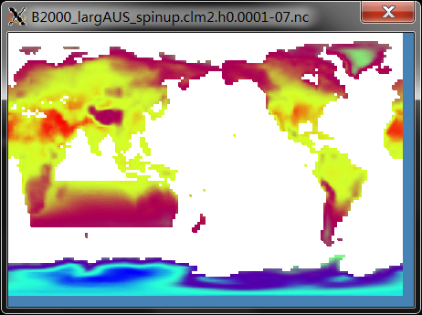
Fig.1 Modified Land/Sea Mask Runtime Demo (Surf Temp in 0001-07)

We expand the land westward based on the natural eastern coastline of Australia (northeast corner: Cape York, and southeast corner: Tasmania), and naturally merged the African continent. For the newly emerged landmass, Plant Functional Types (PFT) are entirely set to bare soil, with the model default clay/sand/silt ratio. Soil color is set to code 20, which is in accordance with the western Australia. The terrain height is 10 m to avoid sea level change issues. We compiled the CAM3.5 physics package to accelerate the model spin-up. With 10 nodes (240 processors) layout on TH-2, CAM3.5 physics gains ~20% speed-up than CAM4 physics (27 sim.y/day vs 22 sim.y/day).

You may check the following links about the land surface properties: GLDAS Soil Land Surface

Also, Please see the previous post about modifications of PFTs and soils in the CLM.

Below we archive the procedures to achieve the goal.

I. Modify Land Sea Mask

We first decide how much we expand the landmass. After that, it would be convenient to use the modified land/sea mask file as a reference to generate other files. All CESM land/sea mask info comes from ocean data. Here we start from the gx1v6_090205.nc. If you are not familiar with this, please refer the previous post.

1. Use python tool to convert land/sea mask to binary map (0-1 bmp) file.

2. Use your GUI tool (even paint app on windows) to edit the land/sea mask to fit your need.

3. Use python tool to convert bmp back to imask ncfile.

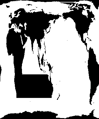
Fig.2 Modified Land/Sea Mask Bitmap (note the ocean grid system gives some deformation look)

II. Ocean

Based on the modified land/sea mask file, we then adjust the corresponding ocean files.

1. Use this script to change bathymetry. Note the “big-enddian/little endian” shift is much easier in python.

2. Check the bathymetry is correctly modified. Here we maintained the original bathymetry to minimize the change in the real ocean (hop the integration is smooth).

3. Change Oceanic Region Mask.

4. Change Initial condition.

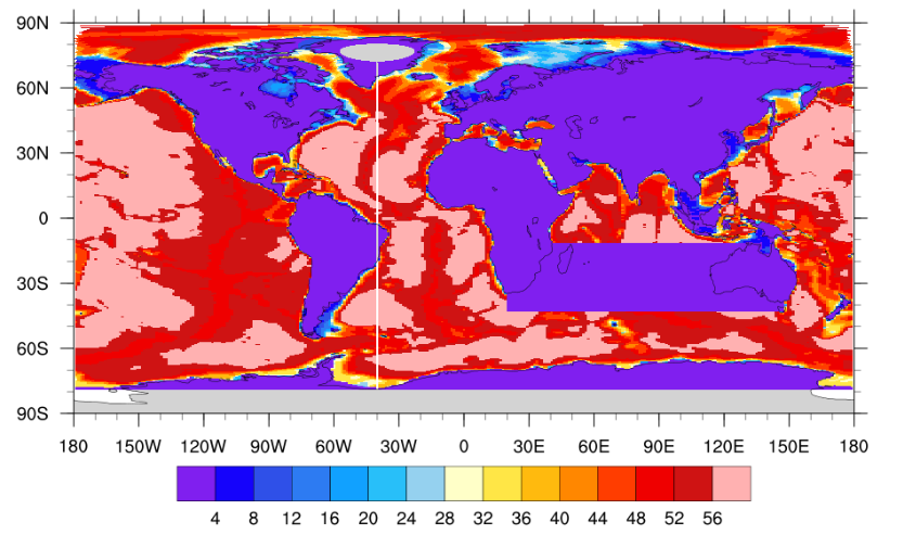
Fig.3 Modified Ocean Bathymetry (shadings denote active grids in one ocean column)

III. Coupler

Follow the previous post to generate SCRIP mapping files and domain files for other components.

IV. Atmosphere

Using the generated domain files, here we modify the topography file for the atmosphere.

1. Use this script to change the LANDFRAC and PHIS (terrain height) in topography file according to the domain.lnd file generated in III. (LANDFRAC is ignored by CAM4 and CAM5; fractional land is defined by the coupler mapping files.)

IV. Land

Use this script to modify the land surface data sets, including PFT, soil color, etc.

V. Namelist

Follow the previous post to setup your namelist files.

VI. Troubleshooting

We can successfully integrate the model after above settings. The question is, we found runtime error from atm model

COLDSST: encountered in cldfrc:         241           6  0.161392688007392

This error comes from cloud_fraction.F90, and it complains about low SSTs. We then found there is a strenge error from cpl to the atm that the grid cell with certain fraction of ocean surface, feels SST=0K. This should not have happened as scrip mapping should have handle it well. We recheced all files with proper configurations and finally used some tricks to get SST from adjacent cell and rewrite the wrongly set SST in the fractional cell.

VII. Combined script

1. Main Driver
2. Cpl Controller
3. Setup Experiment

VIII. Gallery

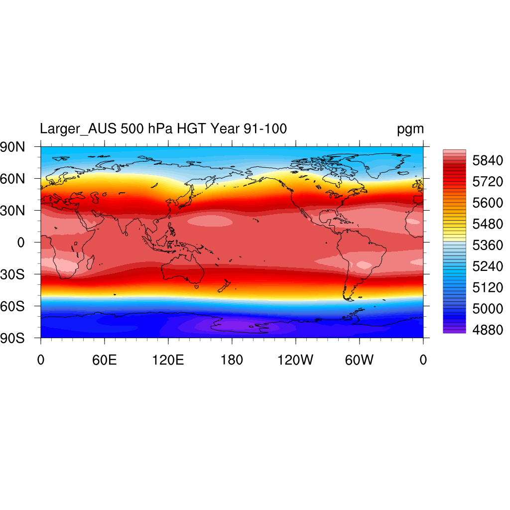
500 hPa HGT

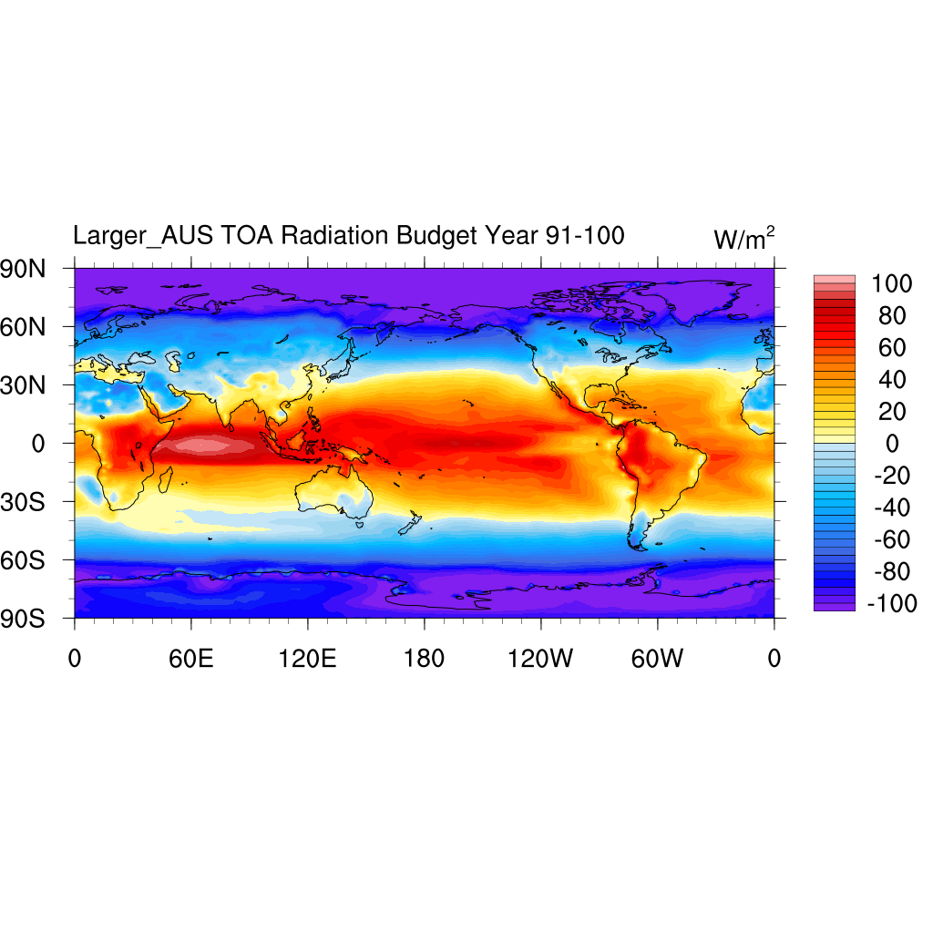
TOA Radiative Budget

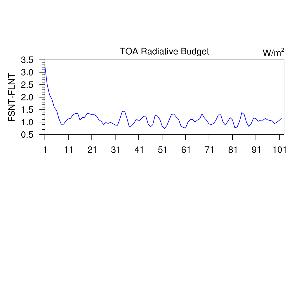
TOA Radiative Budget Time series

Surface Temperature