- I. Build Domains
- II. Build Bathymetry Data
- III. Build ICBC for ROMS by HYCOM output
- IV. Change the maximum current speed limit
- V. SCRIP Weighting File
- VI. Gallery
- Acknowledgement
After Repeating Sandy (2012), we finally come to start to build the coupling framework over the Guangdong-Hong Kong-Macao Greater Bay Area (GBA). Here we archive the process in building the coupling framework for simulating Mangkhut (2018).
The Sandy (2012) case can be smoothly repeated by following the instructions on the manual. While buiding up the coupling framework over the GBA need more efforts.
I. Build Domains
I skipped the WPS procedure for building WRF grid system. Now we form the ROMS grid system using WPS generated geo_em data.
1.1 Use WPS to generate a geo_em file which is equal or larger compared to your aim ROMS domain. For example, in our case, we need to set the ROMS in around 2.2 km spatial resolution and 900x600 size, so I generate a geo_em file with 3 km and 1000x1000 size first.
1.2 Generate ROMS grid system by geo_em from WRF-WPS. There is an urban legend that all islands with sizes smaller than 4 px need to be removed to ensure the smooth run. I even tried Computer Vision algorithm to label the connected components and then remove the elements. Finally, I found this is not necessary. The underlying cause of unstable integration is still from the bathymetry. step1_roms_grid_from_wps_200219.m
Meanwhile, we need to be careful to fit the condition in Lm and Mm:
! Lm           Number of INTERIOR grid RHO-points in the XI-direction for
!                each nested grid, [1:Ngrids]. If using NetCDF files as
!                input, Lm=xi_rho-2 where "xi_rho" is the NetCDF file
!                dimension of RHO-points. Recall that all RHO-point
!                variables have a computational I-range of [0:Lm+1].
!
! Mm           Number of INTERIOR grid RHO-points in the ETA-direction for
!                each nested grid, [1:Ngrids]. If using NetCDF files as
!                input, Mm=eta_rho-2 where "eta_rho" is the NetCDF file
!                dimension of RHO-points. Recall that all RHO-point
!                variables have a computational J-range of [0:Mm+1].
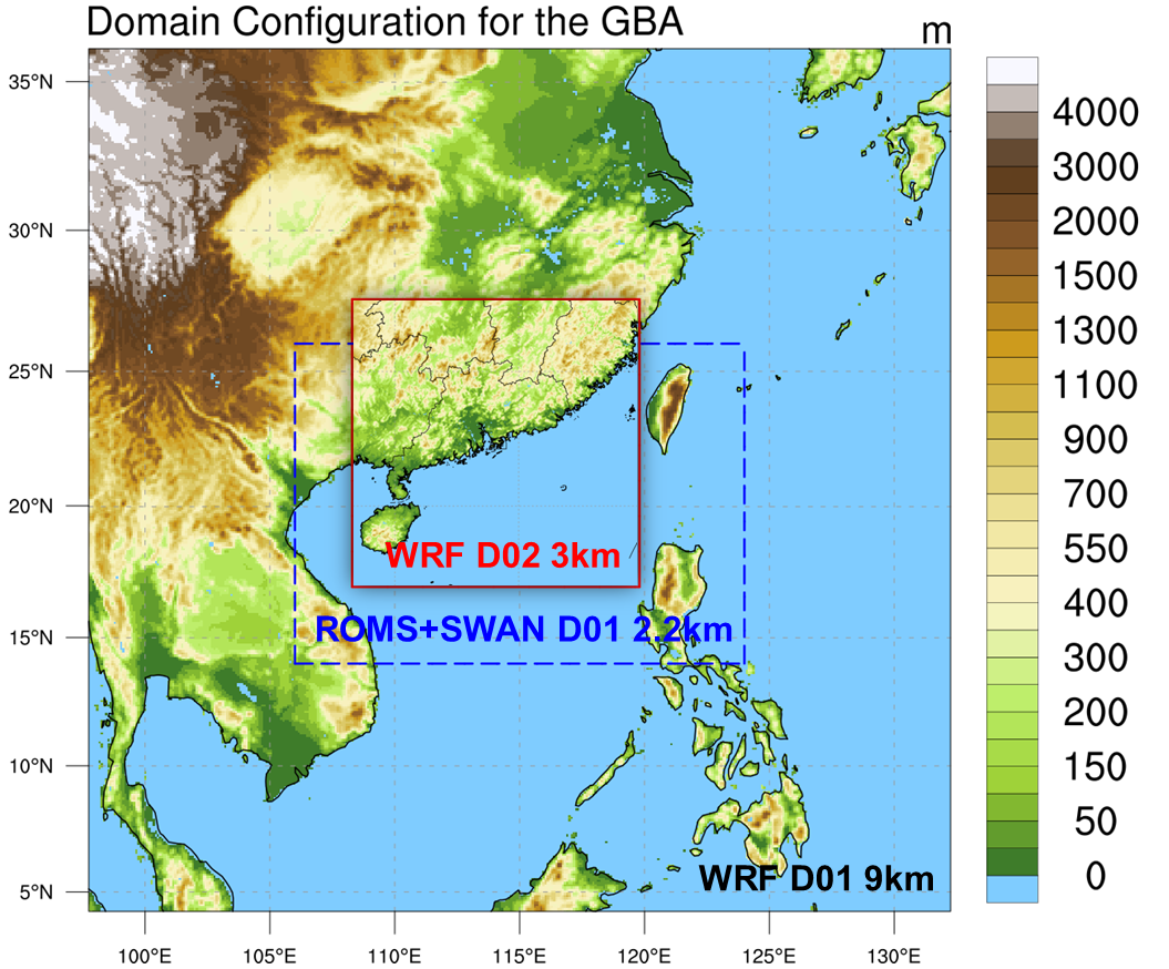
Final Domain Configuration (Outer and white inner box for WRF, and black dashed box for ROMS):
II. Build Bathymetry Data
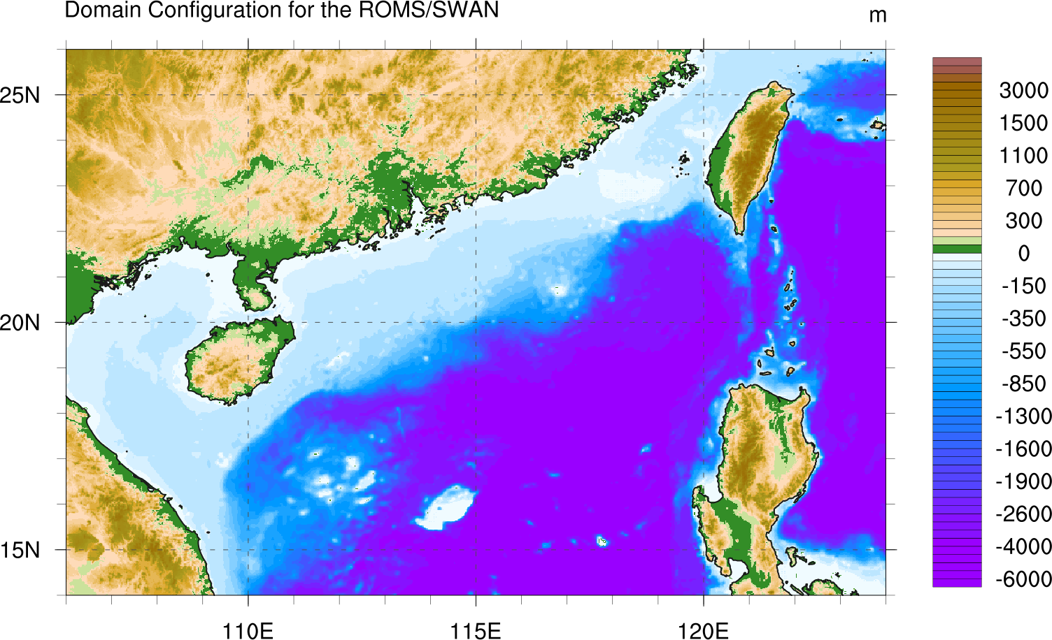
2.1 Use ETOPO bathymetry data to fill the h in the generated file roms_grid.nc. Here we use a simple neighboring method to fill the h in each grid. step2_ETOPO_bath_to_roms_200219.ncl
2.2 Preliminary process the bathy using 9-point smooth. This is optional, as the following LP method is quite effective in optimizing the bathy. Of note is that here we also set the minimum bathy to 10 m. This is quite important as the vertical velocity can easily violate the CFL condition if the shallowest water near the coast is too shallow.
How to justify “too shallow”? In this case, we have a strong typhoon, using 10 s dtime in ROMS, the 10-m shallowest bathy works fine. Meanwhile, we restricted the deepest bathy to 3000 m, as we do not concern the deep sea process in this relative short simulation. step3_OPTIONAL_prim_process_roms_bath_200219.ncl
Original Bathymetry:
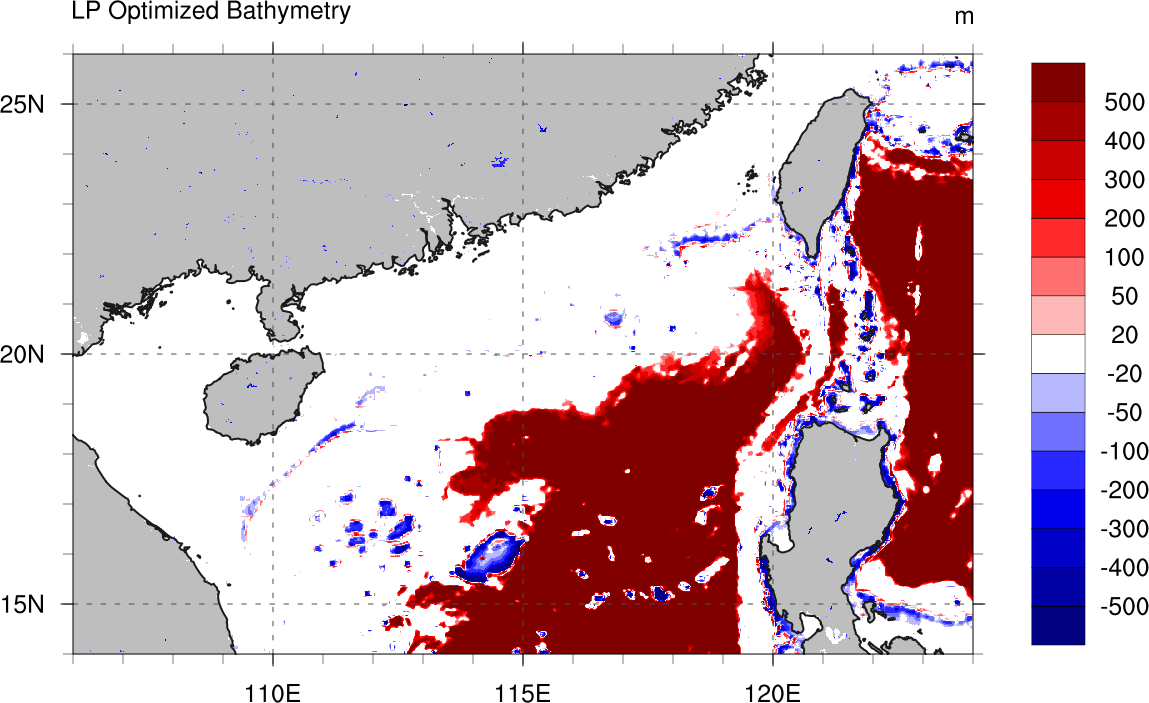
2.3 Smooth the bathemetry to satisfy the rx threshold, using the LP method. There is a toolkit from IRB in Croatia LP Bathymetry, providing several ways to deal with the problem.
Note the lp_solve command line tool need to be installed at frist. For other version, remember to download the file named as lp_solve_x.x.x.x_exe_ux64.tar.gz. step4_LP_smooth_bath_200219.m
Bathymetry Change After LP Optimization. Note that the deepest bathy has been cut off at 3000 meter:
Why/How do we smooth the bathy in ROMS? I quote a very insightful post from the ROMS forum here:
1) compute vertically stable! profile of temp and salt for the domain you are running, horizontally homogeneous! , hence not producing any density gradients. In other words, create ana vertical profile for temp and salt in a similar way as is done for many examples in ana_initial.h . In that way if you start your simulation WITHOUT any forcing! the ocean should stay (not exactly, diffusion etc, but lets pretend it does, with big confidence) in stable state, you have only vertically stable stratified density, not producing any velocity (because there are no density gradients). However we are not on z grid and there is a sigma slope so you will have effects of HPGE, which are direct consequence of “bad” rx1.
In that way you can see what is the effect of “bad bathymetry and big rx1” and where it is introducing artificial currents because of HPGE.
Usually look at the bottom, where pressure builds up.
2) I identify those regions (i.e. using magnitude of velocity) and create weight factor for smoothing, big magnitude big weight. You want to smooth only there where you have big errors from HPGE, and keep as close as possible to real bathy. After smoothing you get new bathy, run the same case again and compute magnitude again, do that in a iterative way until you are happy. In my case I have to run model for a week to get to steady state with “HPGE” currents that are not changing any more.
Also according to Dutour et al. (2009):
The initial error, called an error of the first type (Mellor et al., 1994), is easy to estimate: simply run the model with no forcing and a horizontally uniform vertical T/S profile to get the induced currents. The remaining HPG error, called an error of the second type, is much smaller but still creates artificial currents, which limit the stability of the model. It is very difficult to estimate this error and there are only heuristic rules about it based on experience with the ROMS model. To be on the safe side, it is recommended to use grids with , and most simulations with ROMS are done with and (see Shchepetkin and McWilliams (2003) for more details). Therefore, we call a grid numerically stable if , even if this is somewhat arbitrary. Useful links:
* https://www.myroms.org/forum/viewtopic.php?t=2330
* https://www.myroms.org/forum/viewtopic.php?t=612
III. Build ICBC for ROMS by HYCOM output
Here is a bug in the original mtools from the COAWST if using OPeNDP through the network interface. Thus, we download the HYCOM data manully through a python script, and rewrote some code in the orginal mtool.
3.1 Download HYCOM data. 200211-down-hycom.py
3.2 Interpolate to the model layers. This will take a while. step5_local_gba_roms_master_climatology_coawst_mw_200219.m
IV. Change the maximum current speed limit
In ROMS/Modules/mod_scalars.F, change max_speed = 20.0_dp to max_speed = 100.0_dp as TC may cause very strong surface current.
V. SCRIP Weighting File
Follow the instrucitions in the manual and compile the scrip_coawst util for generating the weighting file. Note that the path in scrip_coawst_XXX.in should not longer than 80 chars.
VI. Gallery
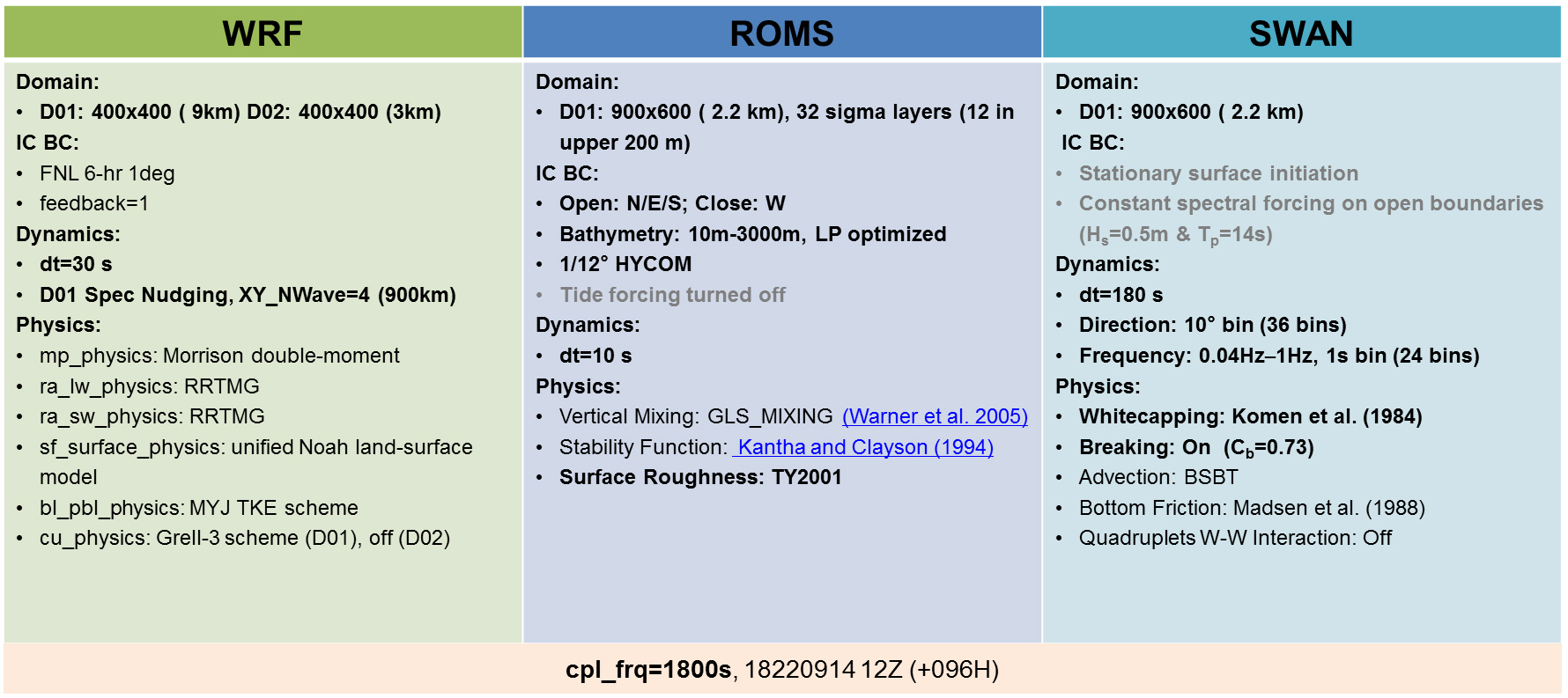
Current settings across 3 component models in the COAWST:
Task-based Load-Balancing Configuration:

The ROMS surf layer temp:
Acknowledgement
We really appreciate Dr. John Warner for his great efforts to build the COAWST coupling framework, which provides us the possibility to investigate our potential ideas in TC-wave-sea simulation. We also appreciate Dr. Mathieu Dutour Sikiric for his LP bathy tool to optimize the bathy over the SCS, which is very important to run the model stably.
Updated 2020-03-17